
Harbir Antil
Recent Research Interests
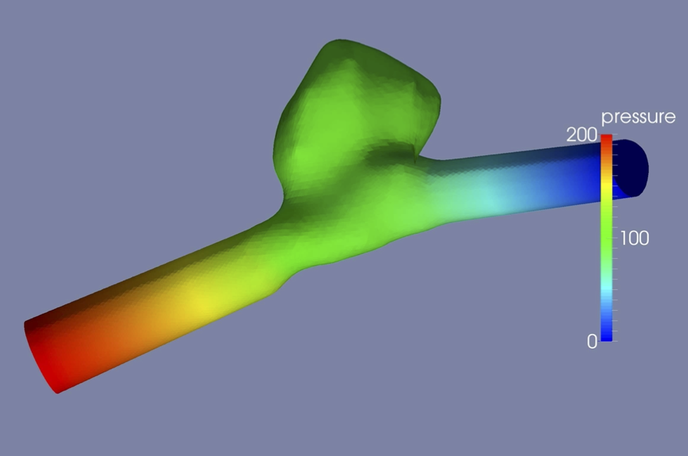
- Fluid dynamics
- Imaging
- PDE-constrained optimization
- Topology optimization
- Shape optimization
- Risk-averse optimization
- Reduced order modeling
- Deep learning
Optimization and Control
Optimization problem with constraints given by partial (ordinary) differential equations (PDEs / ODEs) can be written as
subject to: e(u,z) = 0,
over (u,z) ∈ Uad x Zad.
Here, J: U x Z → ℜ stands for the objective functional depending on the state variables u ∈ U and the control variables z ∈ Z. The equation corresponds to the PDE (linear/nonlinear), and Uad ⊂ U, Zad ⊂ Z refer to the sets of admissible states and control variables, respectively. The variable z could be an optimal control (optimal control problems) or a shape parameter (shape optimization problems).
The numerical solution to PDE constrained optimization problems involves a series of theoretical and practical challenges:
- Solving a PDE constrained optimization problem not only require a solution to state equations but adjoint equations as well.
- The PDEs may not equalities, but could be complementarity problems or variational inequalities. Also, these problems may contain uncertainty due to unknown boundary conditions, coefficients, etc.
- The structural interaction between optimization algorithms and the underlying PDE and the impact of the discretization processes have to be taken into account.
- The numerical approaches typically lead to large-scale nonlinear programming problems. With regard to algorithmic complexity, their numerical solution requires the use of efficient iterative schemes such as multilevel techniques.
- Significant savings both in terms of memory and computational time maybe needed via model reduction techniques.
| [1] | Frontiers in PDE-constrained Optimization. The IMA Volumes in Mathematics and its Applications, Springer 2018. |
Reduced Order Modeling
Consider a linear or nonlinear dynamical system and quantity of interest given by y. We are interested in deriving a reduced order model, which is cheaper and faster to evaluate.
Nonlocal PDEs
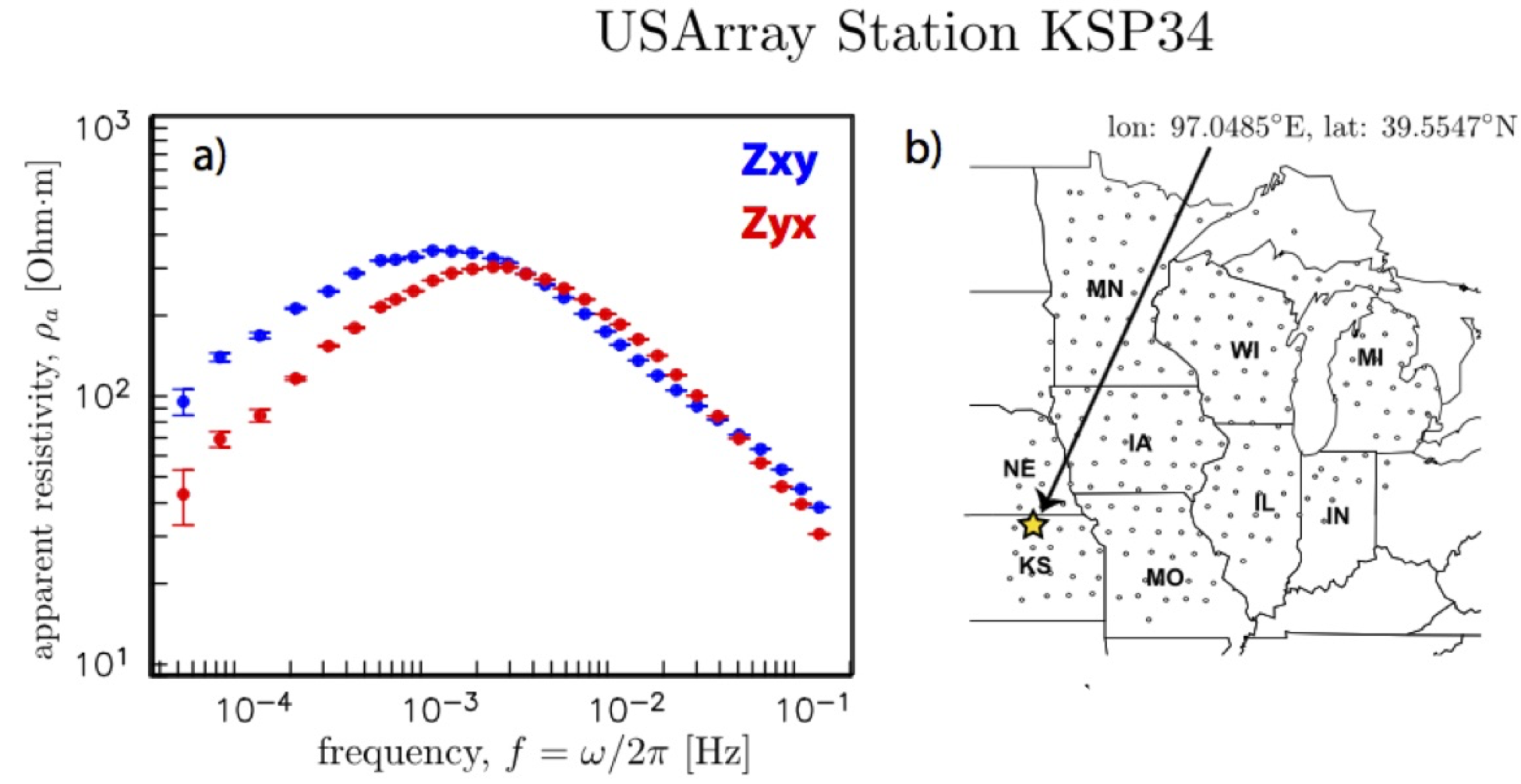
It is becoming clear that the assumptions leading to classical PDE based models are not always accurate or realistic. Fractional models have emerged as a replacement because: they can capture sharp transitions across interfaces and they can capture nonlocal effects. Such problems occur in imaging science and phase field models. The fractional Laplacian has received a tremendous amount of attention partly due to the fact that it is the generator of the Le ́vy process. Surprisingly, the probability community has been using these concepts for several decades. A not so well-known fact is that fractional operators natural arise in the celebrated Haldane-Shastry and Calogero-Moser quantum spin chains models and they are also emerging as a natural candidate for classical Oseen-Frank energy for a nonlocal Liquid crystal model. The nonlocal models are also playing a significant role in geophysical electromagnetics and machine learning. Using the Nonlocal models, it is also possible to introduce novel optimal control concepts, such as exterior optimal control.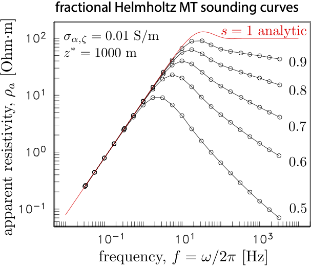
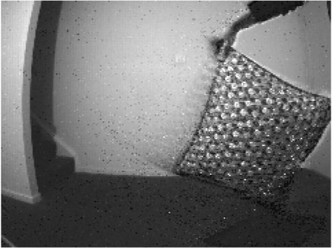
Neuromorphic Imaging
Event or Neuromorphic cameras are novel biologically inspired sensors that record data based on the change in light intensity at each pixel asynchronously. They have a temporal resolution of microseconds. This is useful for scenes with fast moving objects that can cause motion blur in traditional cameras, which record the average light intensity over an exposure time for each pixel synchronously. In our work, we consider bilevel optimization based variational framework for neuromorphic imaging.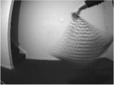
Deep Neural Networks
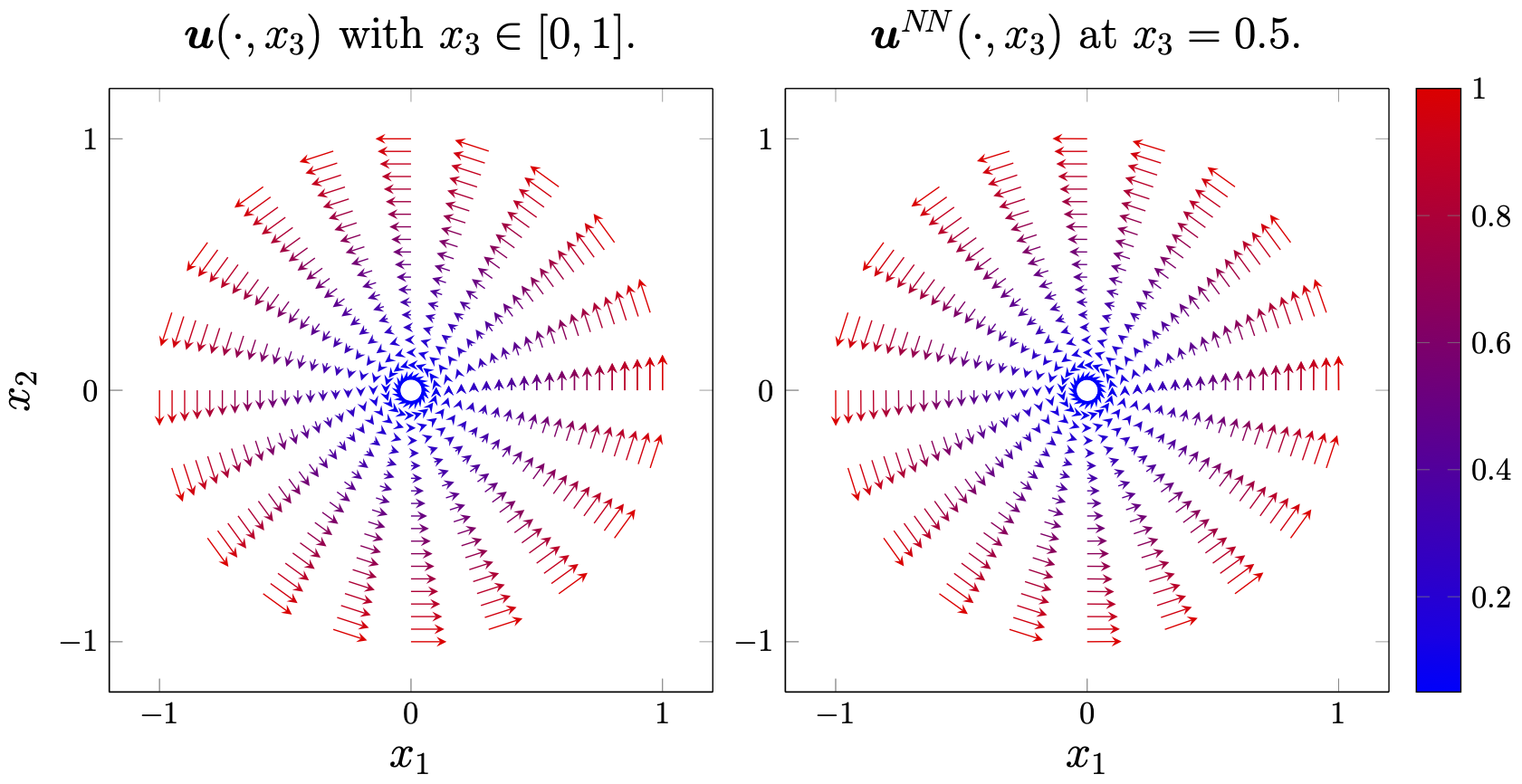
Our group’s work on deep neural networks (DNNs) focuses on writing DNNs as constrained optimization problems. In particular, we have introduced DNNs with memory, which helps overcome the vanishing gradient challenge. We have also explored reducing the computational complexity of DNNs by introducing a bias ordering. These proposed DNNs have been shown to be excellent surrogates to parameterized (nonlinear) partial differential equations (PDEs), Bayesian inverse problems, and data assimilation problems, with multiple advantages over the traditional approaches. We have applied these DNNs to chemically reacting flow problems. The latter requires solving a system of stiff ODEs and fluid flow equations. These are highly challenging problems, for instance, for combustion the number of reactions can be significant (over 100). Due to the large CPU requirements of chemical reactions (over 99% of total CPU time), a large number of flow and combustion problems are presently beyond the capabilities of even the largest supercomputers.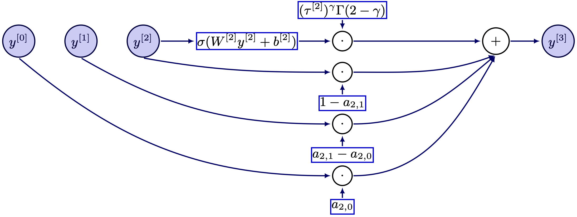
Current Projects
Selected research grants, see Curriculum Vitae (.PDF) for more details.Current
-
National Science Foundation (NSF) DMS - 2408877
Structure Preserving Optimization Algorithms and Digital Twins.
August 2024-July 2027. -
Air Force Office of Scientific Research (AFOSR) - FA9550-24-1-0022.
Defense University Research Instrumentation Program (DURIP).
Optimization for Neuromorphic Imaging and Digital Twins.
April 1, 2024 - March 31, 2025. -
Office of Naval Research (ONR) - N00014-24-1-2147
Efficient Algorithms for Optimizatoin with PDE Constraints.
February 2024-January 2029. -
National Science Foundation (NSF) DMS - 2330895 (together with Benjamin Seibold (Temple) and Kathrin Semtana (Stevens))
Mathematical Opportunities in Digital Twins.
August 2023-July 2024. - Air Force Office of Scientific Research (AFOSR) - FA9550-22-1-0248.
Compression and Randomization for Extreme-Scale Training & Optimization (CREST Opt).
May 2022-April 2025. -
National Science Foundation (NSF) DMS - 2110263
Algorithms and Numerics for Optimization Problems with PDEs.
August 2021-July 2025.
Past projects
- DARPA (together with Tyrus Berry)
Geometries Of Learning (GoL).
April 2022-August 2023.National Science Foundation (NSF) DMS - 2110263 (together with Pablo Stinga)
Nonlocal School on Fractional Equations.
June 2022-May 2023. - Defense Threat Reduction Agency (DTRA) (together with Rainald Loehner)
Numerically Inspired Deep Neural Nets for Chemically Reacting Flows (NINNs).
April 2022-October 2022. - Air Force Office of Scientific Research (AFOSR) - FA9550-21-1-0181.
Defense University Research Instrumentation Program (DURIP).
Optimization, Control, Networks and Learning from Data.
May 2021-October 2022. - Defense Threat Reduction Agency (DTRA) (together with Rainald Loehner).
Neural-Net/Deep Learning Based Chemical Reaction Package.
April 2020 - September 2022. - National Science Foundation (NSF) DMS - 1913004
Collaborative Research: Multilevel Methods for Optimal Control of Partial Differential Equations and Optimization-Based Domain Decomposition.
July 2019-June 2022. -
National Science Foundation (NSF) DMS - 1907412
East Coast Optimization Meeting (ECOM).
March 2019-August 2022. - Air Force Office of Scientific Research (AFOSR) - FA9550-19-1-0036.
Structure Exploiting Trust Regions for Bilevel and Risk-Averse Optimization.
January 2019-December 2021. - Department of Navy, Naval PostGraduate School - N00244-20-1-0005.
Constrained Optimization and Machine Learning.
February 2020 - February 2022. -
National Science Foundation (NSF) DMS - 1818772
Partial Differential Equation Constrained Optimization: Algorithms, Numerics, and Applications.
August 2018-July 2021. - National Institute of Standards and Technology (NIST).
Algorithms for Image and Shape Analysis in 3d.
August - December 2020. - Department of Energy, Sandia National Laboratories
Fractional differential operators for features detection in the subsurface.
January-May 2019. - Department of Energy, Sandia National Laboratories
Fractional operators in Geophysics.
January-May 2018 -
National Science Foundation (NSF) DMS - 1521590
Numerical Analysis of Partial Differential Equation Constrained Optimization Problems.
July 2015-May 2019.
Outcomes
- See Publications for a complete list of latest work
- Software written link
- Mentoring of students and postdocs link